Regression analysis seasonal 6.0
Summary
This operator calculates a regression model for a time series. The regression model tries to explain observations with the help of trends, seasonal variations and other influencing factors, and creates a forecast for future dates.
A time series is a sequence of data points, measured typically at successive times spaced at uniform time intervals [1], e.g., temperature measured at every hour or weekly sales figures.
The seasonal regression model allows also to analyze whether the observed data depend on other influencing factors (e.g., training, marketing campaigns, number of employees).
A detailed description of regression analysis methods can be found at [2].
Requirements for data to be analyzed
- Input data must be scaled, i.e., the time stamps in columns 'Date + time (from)' and 'Date + time (to)' represent uniform time intervals of the same duration. (see Scaling 7.0)
- Input data must be sorted by time stamps in the columns 'Date + time (from)' and 'Date + time (to)'.
- The columns 'Date + time (from)' and 'Date + time (to)' must not contain missing entries.
- The underlying data must comprise at least one complete season.
- If one or several observations are missing, the corresponding time stamps will be inserted into the data. The inserted entries are treated as missing observations.
Please note
- Additional information, such as training and validation errors, and warnings are reported in the description field of the operation within the TIS-GUI.
- If the column of an influencing factor contains the same constant value for each observation no regression analysis can be carried out. Thus, constant factors are excluded automatically.
Example: Regression model with trend and season
Situation |
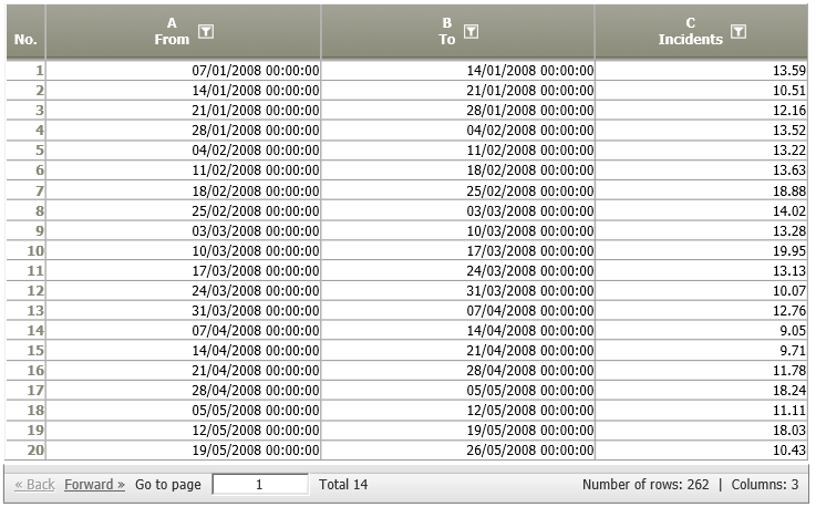
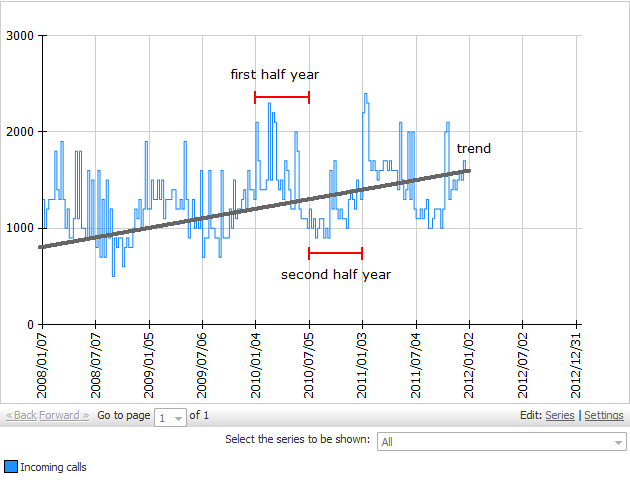
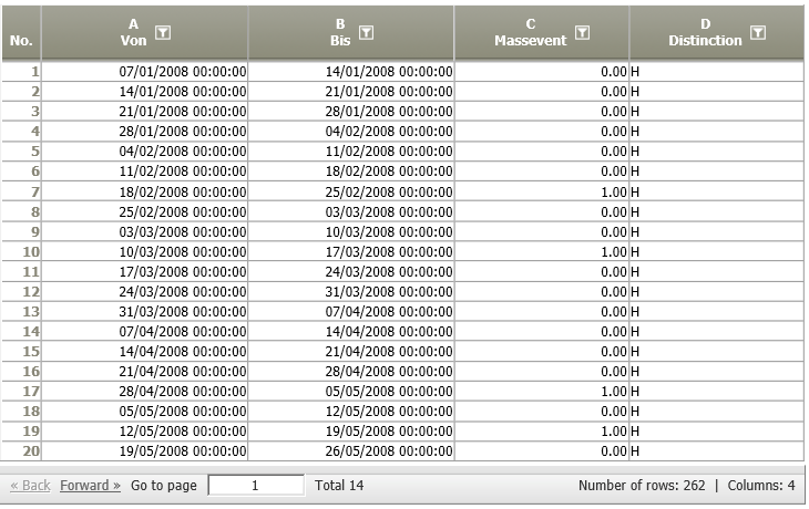
We consider the number of incoming phone calls at a call center over a period time. More precisely, we are given the number of incoming calls for each single week during the last four years.
|
|---|---|
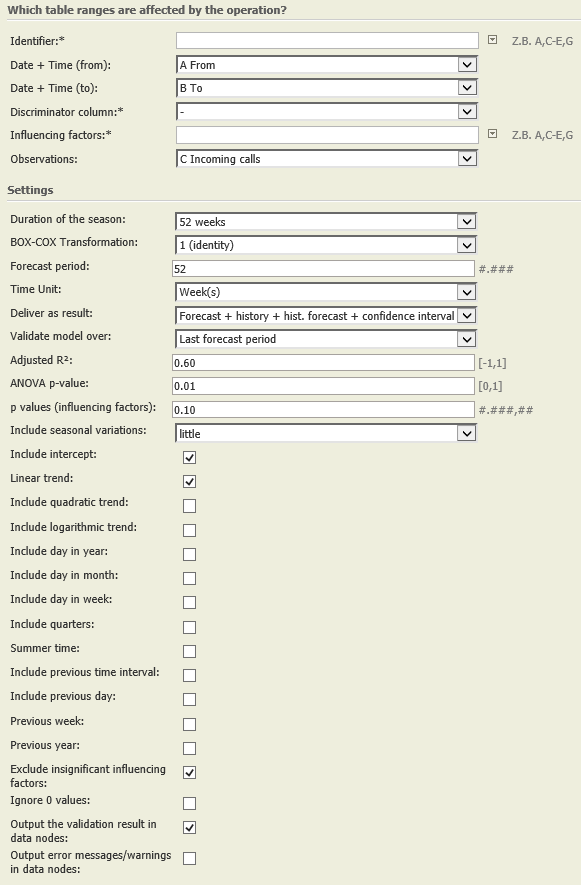
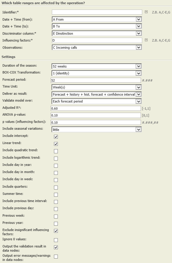
Settings |
|
Result |
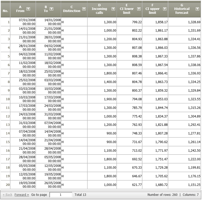
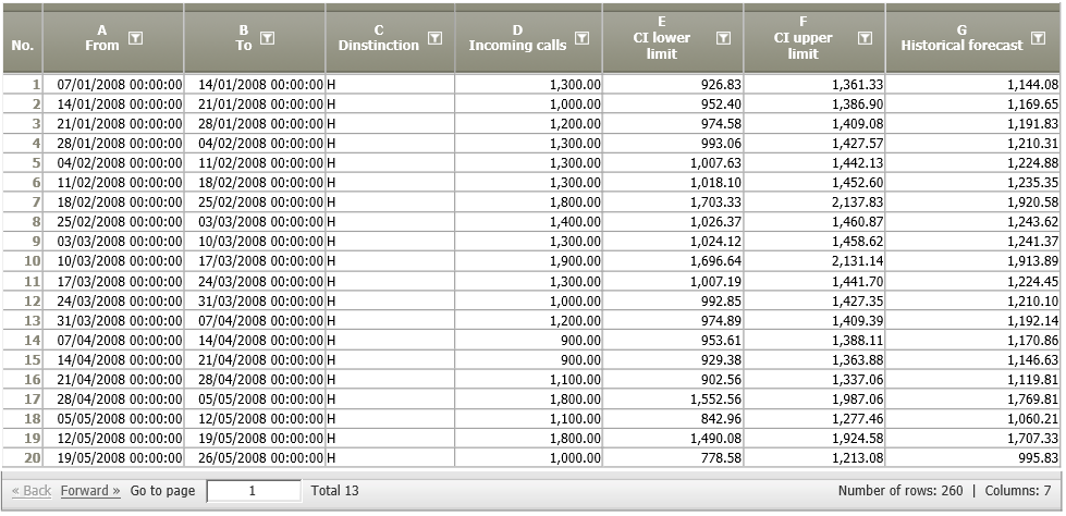
The resulting data node shows the forecast (G), and the lower and upper limits of the confidence intervals (E and F).
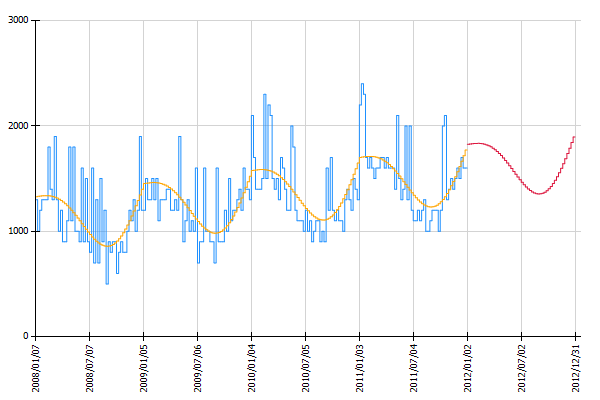
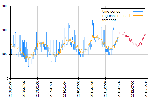
By adding a chart operation Chart: Histogram Time Pattern the visualization shows that the historical forecasts (orange line) estimated with the obtained regression model show a similar trend and seasonal behaviour as the historic observations (blue line). The red line shows the estimated number of phone calls for the next 52 weeks.
|
Project-File |
Want to learn more?
Settings
This operator calculates a regression model for a time series. The regression model tries to explain observations with the help of trends, seasonal variations and other influencing factors, and creates a forecast for future dates.
Columns of input table
Parameter
Examples
Example 2: Regression model with trend, season and influencing factors
Situation |
On the basis of that modified input we can now build an extended regression model. We specify advertising campaigns as an addtional influencing factor and the distinction column in the settings of the regression operation. |
|---|---|
Settings |
|
Result |
The resulting data node shows the forecast (G), and the lower and upper CI limits (E, F).
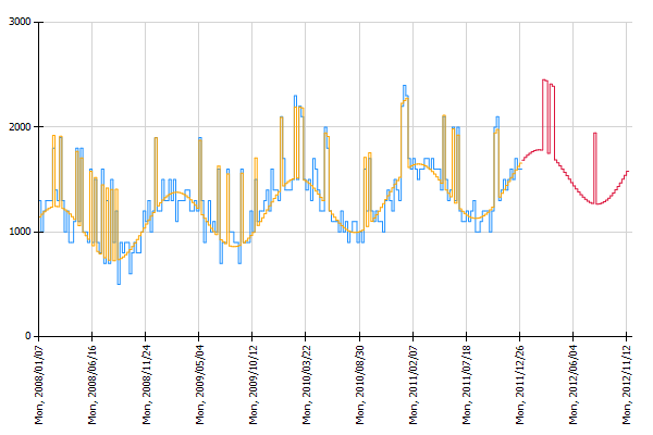
In the histogram visualizing the results (added with the operation Chart: Histogram Time Pattern) we see that campaigns could indeed explain an increased number of incoming calls in the past (compare orange and blue line). Also the forecast for the next 52 weeks (red line) contains high values whenever an advertising campaign will be run.
|
Example 3: Comparison of different regression models
Situation |
To be able to compare two or several regression models with each other, operation regression analysis 6.0 validates each model in the following manner.
|
|---|---|
Settings |
|
Result |
If we consider and compare the validation error associated with the two models from example 1 and example 2 we see that the validation error could be reduced by including advertising campaigns within the model for example 2. In general, one regression model should be preferred against the other only if it has a significantly lower validation error. |
Example 4: Analyzing hourly and daily data over a long period of time
Situation |
When analyzing hourly or daily data over a long period of time it is advisable to split your data into several groups and carry out a regression analysis for each group seperately. |
|---|---|
Settings |
For example, if daily data shall be forecasted, a column needs to be created containing the weekdays using the Formula operator (row-by-row) (4.0) = Formeloperator. Settings are shown in the figure below: If the forecast shall be at hourly intervals, the formula operator settings are: Afterwards, to carry out a regression analysis for each group separately, you have to specify the previously introduced column in the field "Identifier" within the settings of the operation regression analysis 6.0 |
Troubleshooting
Problem |
Frequent Cause |
Solutions |
|---|---|---|
Error message: "Object reference not set to an instance of an object." |
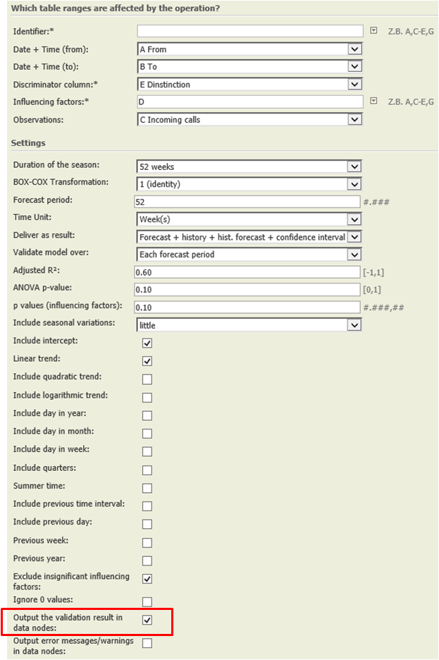
in TIS 5.8.2, this error message occurs when the box "Output the validation result in data nodes" is checked. This is a bug, see ticket |
... |
Forecast for excluded days, e.g., holiday. |
The operator does not consider if a day in the future period is a day to be excluded or not. In our TIS Forecast solution not additional influcencing factors for days to be exlcuded are provided. If a regression model is based on at least of these influencing factor, the forecasted value for that day will be null. If a regression model does not use any additional influencing factors, e.g., they are all elminated due a high p-value, then will be a forecasted value for an excluded day. |
In the TIS forecasting solution those forecasted rows representing excluded days will be eliminated after the regression forecast (merge data, rows without a common key in data node 2). |
Related topics
- ...

