TIS 6 User's Manual

Summary

This operator creates a seasonal ARIMA model for time-related observations. A forecast is created with the help of this model.

In time series analysis, an autoregressive integrated moving average (ARIMA) model is a generalization of an autoregressive moving average (ARMA) model. These models are fitted to time series data either to better understand the data or to predict future points in the series (forecasting). They are applied in some cases where data show evidence of non-stationarity, where an initial differencing step (corresponding to the "integrated" part of the model) can be applied to reduce the non-stationarity (wikipedia).

Configuration

Input settings of existing table

Name	Value	Opt.	Description	Example
Identifier	System.Object	opt.	Please select those columns based upon whose content the data should be grouped. A separate seasonal ARIMA analysis will be conducted for each group.	-
Date + Time (from)	System.DateTime	-	Please select the column that contains the start times (date + time) of your observations.	-
Date + Time (to)	System.DateTime	-	Please select the column that contains the final times (date + time) of your observation.	-
Observations	System.Double	-	Please select the column which contains the observations relevant for the seasonal ARIMA analysis.	-

Settings

Name	Value	Opt.	Description	Example
Ignore 0 values	System.Boolean	-	Rows with 0-values are ignored in the seasonal ARIMA model and are treated like missing data.	-
Duration of the season	System.String 1 year 52 weeks 1 week 3 months 1 month 1 day 12 hours 8 hours 6 hours 1 hour	-	Please enter the duration of the season (=number of the data/observations/values of a season). The duration of the season must be equal to or greater than one.	-
Basic model	System.String 001 011 101 110 111	-	Please select the type of ARIMA process for the basic model. A model that can be applied to a great deal of data is a basic model=011, seasonal model=011. This model corresponds to the Holt winter seasonal method.	-
Seasonal model	System.String 000 001 011 101 110 111	-	Please select the type of the ARIMA process for the seasonal model. A model that can be applied to many kinds of data is basis model=011, seasonal model=011. This model corresponds to the Holt winter seasonal method.	-
@BOXCOXTRANSFORMATION	System.String Automatic 1 (identity) 0.5 (root) 0 (logarithm) -1 (reciprocal value)	-	The BOX-COX transformation transforms the observations into a form that can be used for the seasonal ARIMA analysis. If you select 'automatic' as the type of BOX-COX transformation, a transformation suitable for the data on which the analysis is based is defined. Another type of transformation should then only be used if you have sound knowledge of the data to be analysed. Select '1 (identity)', if the seasonal variations remain absolutely constant, e.g. the December value is always 1000 units higher than the annual average. Select '0 (logarithm)', if the seasonal variations are a constant percentage, e.g. the December value is always 20% higher than the annual average. Select '0.5 (root)', if the seasonal variations are a constant percentage, but the percentage reduces slightly over time, e.g. the first December value is 20% higher than the monthly average, the second December value is 19% higher, etc. Select '-1 (reciprocal)' for non-negative data with falling trend, for example, as for sales data from a bookshop/publishers, where high figures are observed for the first few months after publication, but then gradually reduce over time.	-
Forecast period	System.Int32	-	Please enter the period, e.g. the next 6 weeks, for which a forecast is to be calculated.	-
Time Unit	System.String Year(s) Month(s) Week(s) Day(s) Hour(s)	-	Please enter the period, e.g. the next 6 weeks, for which a forecast is to be calculated.	-
Period for historic forecast	System.Int32	-	Please enter the period, e.g. the last 6 weeks, for which a historical forecast is to be calculated.	-
Time Unit	System.String Year(s) Month(s) Week(s) Day(s) Hour(s)	-	Please enter the period, e.g. the last 6 weeks, for which a historical forecast is to be calculated.	-
Deliver as result	System.String @Forecast Forecast + History Forecast + hist. forecast Forecast + history + hist. forecast + confidence interval Only parameter estimation	-	Please select which data should be displayed in the results.	-
Show estimated parameters	System.Boolean	-	If selected, the following estimated parameters of the seasonal ARIMA model will be displayed: Lambda (BOX-COX transformation), AR-basis, MA-basis, AR-season, MA-season.	-
Show ACF vector of the residues	System.Boolean	-	If selected, the estimated vector of the auto-correlation function of the residues will be displayed (Lag 1 - Lag 25).	-
Output the validation result in data nodes	System.Boolean	-	If selected, the validation results are displayed in a separate data node.	-
Output error messages/warnings in data nodes	System.Boolean	-	If selected, error messages and warnings are displayed in a separate data node.	-

Want to learn more?

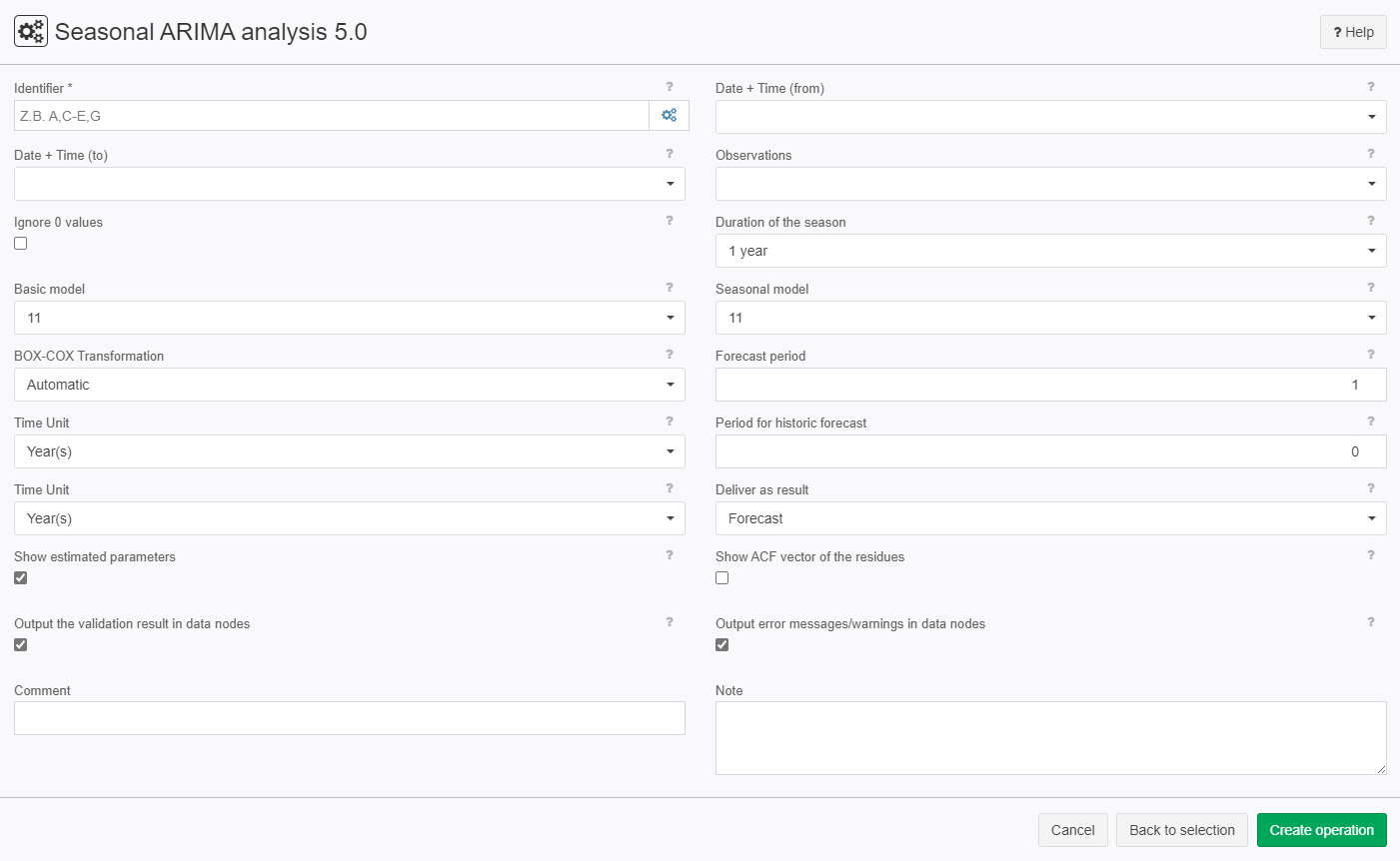
This operator creates a seasonal ARIMA model for time-related observations. A forecast is created with the help of this model.

More detailed information

Data requirements

Input data always need to be sorted by time stamps in column "Date + time". SARIMA Analysis cannot be conducted if this is not the case.
There always need to be 1 season + 1 observation to conduct SARIMA analysis. It does not make sense to calculate a SARIMA model with less data.
Missing time stamps in the input data will be completed as missing rows and treated as missing observations.

Using SARIMA

The TIS-GUI and the SARIMA operator description provide additional information and (if necessary) warnings.

To calculate an ARIMA analysis without seasonality, please choose 000 as seasonal model and 1 as duration of the season.
Days known to be 0 (e.g., Sundays in retail) should be excluded BEFORE from the time series data.

Statistical info

It is difficult to calculate several periods into the future. If you want to forecast further, calculate on an aggregated level (e.g., with weeks instead of days). This will have the disadvantage of losing information, though.
For some data it makes sense to use Autoregression = 2 or Moving Average = 2. However, this leads to slow parameter estimation and rarely provides much better forecasts. Therefore, these models are not provided in TIS at the moment. They can, however, be provided on demand.
Hint: Random Walk = AR1 processes with coefficient 1; this means: the basic model 010 without seasonality. Since no parameter needs to be estimated in the random walk model, and forecast is simply the last observation, this model cannnot directly be chosen. A random walk modell can be estimated by chosing e.g. basic model 011 and seasonal model 000, and the estimated parameter is very close to 0.
Autocorrelation function of residuals = ACF Auto Correlation Function
- e.g. Value = 0.7 ... shows that the model does not fit
- e.g. ABS(x) <0.15 indicates a good model
Parameter estimation in TIS is based on MLE (Maximum Likelihood Estimation)

Examples

Example: Estimating a SARIMA model

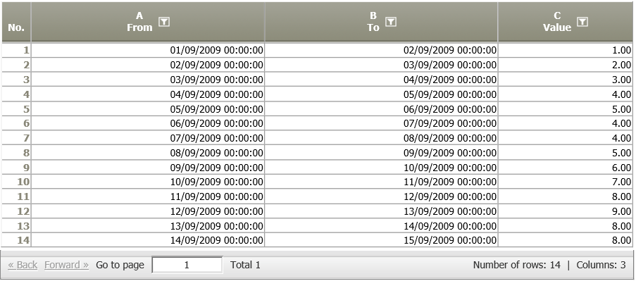
Situation	A value is measured across 14 days. The data show that the value increases by 1 each day and decreases by 1 on the seventh day.
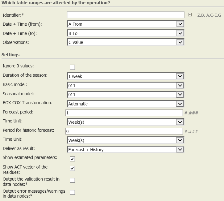
Settings	Add the operation "Seasonal ARIMA Analysis 5.0" to the data node. Enter the settings shown below. We want to see both historical and forecast data in the resulting data node, therefore we chose "Forecast + History" to deliver as result.
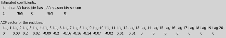
Result	The data node shown below is the result of the SARIMA analysis. The first 14 rows are the observed values (history) and are therefore indicated by an "H". The following 7 rows are the forecasted values and therefore indicated by "F". The operator settings show also the parameter estimates for Lambda (BOX-COX Transformation), coefficients for AR- and MA-processes of the basic and seasonal model. Additionally, the estimated ACF vector of the residues is shown. 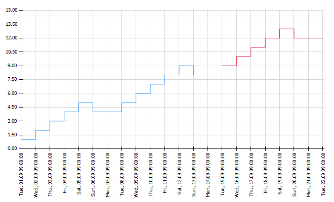To visualize the results, e.g., in a chart, please add a new data node with the operation Chart: Histogram Time Pattern. The result will look similar to the chart below.
Project-File	Confluence Op SARIMA.gzip

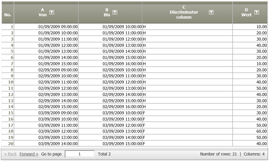
Example: SARIMA model with hourly interval data

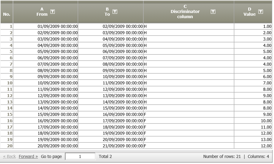
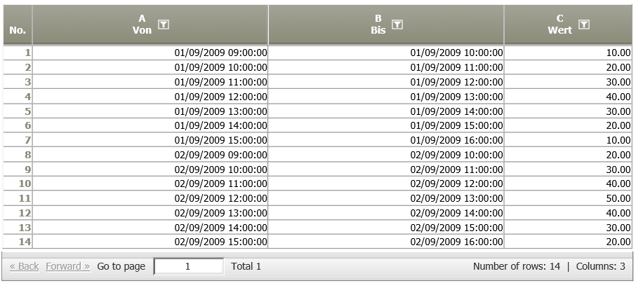
Situation	On two subsequent days, a value is measured each hour in the time between 09:00 to 15:00 hours.
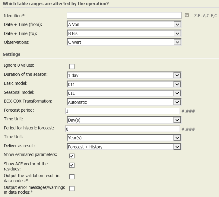
Settings	Add the operation "Seasonal ARIMA Analysis 5.0" to the data node. Enter the settings shown below. We want to see both historical and forecast data in the resulting data node, therefore we chose "Forecast + History" to deliver as result.
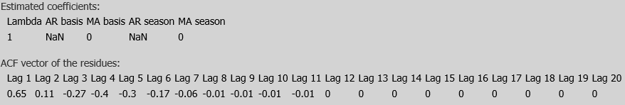
Result	The data node shown below is the result of the SARIMA analysis. The first 14 rows are the observed values (history) and are therefore indicated by an "H". The following 7 rows are the forecasted values and therefore indicated by "F". The operator settings show also the parameter estimates for Lambda (BOX-COX Transformation), coefficients for AR- and MA-processes of the basic and seasonal model. Additionally, the estimated ACF vector of the residues is shown.

Troubleshooting

Problem

Frequent Cause

Solutions

Error message, or "n. def."

The error can be caused by the raw data of the combination of identifiers.

E.g., there are too few values to calculate a certain figure.

Create larger groups, i.e., less filtering by identifier instances.