Regression analysis seasonal 8.0
Summary
This operator calculates a regression model for a time series. The regression model tries to explain observations with the help of trends, seasonal variations and other influencing factors, and creates a forecast for future dates.
A time series is a sequence of data points, measured typically at successive times spaced at uniform time intervals [1], e.g., temperature measured at every hour, or weekly sales figures.
The seasonal regression model allows also to analyze whether the observed data depend on other influencing factors (e.g., training, marketing campaigns, number of employees).
A detailed description of regression analysis methods can be found at [2].
Requirements for data to be analyzed
- Input data must be scaled, i.e., the time stamps in columns 'Date + time (from)' and 'Date + time (to)' represent uniform time intervals of the same duration. (see Scaling 8.0)
- Input data must be sorted by time stamps in the columns 'Date + time (from)' and 'Date + time (to)'.
- The columns 'Date + time (from)' and 'Date + time (to)' must not contain missing entries.
- The underlying data must comprise at least one complete season.
- If one or several observations are missing, the corresponding time stamps will be inserted into the data. The inserted entries are treated as missing observations.
Configuration
Input settings of existing table
Name |
Value |
Opt. |
Description |
Example |
|---|---|---|---|---|
Identifier |
System.Object |
opt. |
Columns by whose content the data is to be grouped. A separate regression analysis is performed for each group. |
- |
Date + Time (from) |
System.DateTime |
- |
Column containing the start times (date + time) of the observations. |
- |
Date + Time (to) |
System.DateTime |
- |
Column containing the end times (date + time) of the observations. |
- |
Distinction History (H) / Forecast (F) |
System.String |
opt. |
This column distinguishes observations from history from observations in the forecast period. Observations from history are marked with "H", observations in the forecast period with "F". This column only needs to be specified if the regression model contains an independent variable. |
- |
Influencing factors |
System.Object |
opt. |
These columns represent those factors which influence the measured observations. The regression analysis tries to establish a (linear) relationship between these factors and the observations. These columns must not include more than one non-numerical column, which contains precisely two different values. These two values are 0-1 coded.
|
- |
Observed values |
System.Double |
- |
This (numeric) column contains the values, which have been observed in each interval of the time series on which the model is based. |
- |
Settings
Name |
Value |
Opt. |
Description |
Example |
|---|---|---|---|---|
Duration of the season |
System.String
|
- |
Please enter the duration of the season on which your data is based. |
52 weeks |
Box-Cox transformation |
System.String
|
- |
The BOX-COX transformation converts the observations into a form that can be used for the regression analysis. If you select 'automatic' as the type of BOX-COX transformation, a suitable transformation for the data on which the analysis is based is defined. Another type of transformation should then only be applied if you have sound knowledge of the data to be analysed. Select '1 (identity)', if the seasonal variations remain absolutely constant, e.g. the December value is always 1000 units higher than the annual average. Select '0 (logarithm)', if the seasonal variations are a constant percentage, e.g. the December value is always 20% higher than the annual average. Select '0.5 (root)', if the seasonal variations are a constant percentage, but the percentage rate reduces slightly over time, e.g. the first December value is 20% higher than the monthly average, the second December value is 19% higher, etc. Select '-1 (reciprocal)' for non-negative data with falling trend, for example, as for the sales data from a book shop, where high values are observed during the first few months after publications, but then fall with time. |
Automatic |
Forecast period in time units |
System.Int32 |
- |
Please enter the period, e.g. the next 6 weeks, for which a forecast is to be calculated. |
26 |
Time Unit |
System.String
|
- |
Please enter the period, e.g. the next 6 weeks, for which a forecast is to be calculated. |
Weeks(s) |
Show in result table |
System.String
|
- |
Please select which data should be displayed in the results. |
Forecast + History |
Model validation period |
System.String
|
- |
The observations are divided into a validation period and training period, e.g. validation period = the last 52 weeks of the data on which the model is based, training period = all other data. A regression model is created on the basis of the training period, and this model is used to estimate the data of the training and validation period. The percentage and average errors between the estimated and actual observations are determined for the training and validation period. If the errors for the training and validation period are very different, your regression model contains too many variables and returns inaccurate forecasts (overfitting). In this case, please try to simplify your model by removing one or more variables. |
Each forecast period |
p-value upper limit |
System.Double |
- |
The p value of an independent variable provides information about whether the observations on which the data is based depends on any of these variables or not. Low values (e.g. less than 0.05) indicate a relationship between independent and dependent variables, high values on the other hand indicate that there are no relationships whatsoever. In this field, please enter a limit for the p value of a single independent variable. If the p value exceeds this limit, this variable will automatically be excluded from the regression model, provided you have activated 'excluded variables'. |
0.05 |
Account for seasonal variations |
System.String
|
- |
The regression model tries to identify seasonal variations and to take these into account for the forecast.
|
middle |
Result column name for upper limits of confidence intervals |
System.String |
Name of the result column containing the upper limits of the confidence intervals. In order to avoid this column to be renamed when the user language or the project language is changed, a custom name, which will remain unchanged, can be entered here. |
CI upper limit |
|
Result column name for lower limits of confidence intervals |
System.String |
Name of the result column containing the lower limits of the confidence intervals. In order to avoid this column to be renamed when the user language or the project language is changed, a custom name, which will remain unchanged, can be entered here. |
CI lower limit |
|
Include intercept |
System.Boolean |
- |
Please do not close the point of intersection unless you are really sure that it does not play any role in your observations. |
True |
Include linear trend |
System.Boolean |
- |
The regression model contains a linear trend, i.e. the observed values rise/fall linearly along the time axis.
|
True |
Include quadratic trend |
System.Boolean |
- |
The regression model contains a quadratic trend, i.e. the observed values rise/fall quadratically along the time axis. |
False |
Include logarithmic trend |
System.Boolean |
- |
The regression model contains logarithmic trend, i.e. the observed values rise/fall logarithmically along the time axis. |
False |
Include calendar day |
System.Boolean |
- |
The location of a date within the year is taken into account in the regression model, e.g. 3.1.2010 is the third day of the year. |
False |
Include day in month |
System.Boolean |
- |
The location of a date within the month is taken into account in the regression model , e.g. 3.1.2010 is the third day in January. |
False |
Include day in week |
System.Boolean |
- |
The effect of different week days is taken into account in the regression model. |
False |
Include quarters |
System.Boolean |
- |
Quarterly periods are taken into account in the regression model. |
False |
Include daylight saving time |
System.Boolean |
- |
Summer time is taken into account in the regression model. |
False |
Include values of previous time interval |
System.Boolean |
- |
The regression analysis examines, whether observations in your previous observations are affected in the scale. |
False |
Include values of previous day |
System.Boolean |
- |
The regression analysis examines whether observations are affected by the observations on the previous day. |
False |
Include values of previous week |
System.Boolean |
- |
The regression analysis examines whether observations are affected by the observations in the previous week.
|
False |
Include values of previous year |
System.Boolean |
- |
The regression analysis examines whether observations are affected by the observations in the previous year. |
False |
Exclude non-significant influencing factors |
System.Boolean |
- |
Influencing factors whose p values exceed the limit given in the 'p values field (influencing factors)' will be excluded from the regression model.
|
True |
Ignore 0 values |
System.Boolean |
- |
Rows with 0 values are ignored and are treated like missing data. |
False |
Show validation result in separate data node |
System.Boolean |
- |
If selected, the validation results are displayed in a separate data node. |
False |
Show error messages/warnings in separate data node |
System.Boolean |
- |
If selected, error messages and warnings are displayed in a separate data node. |
False |
Remarks
- Additional information, such as training and validation errors, and warnings, are reported in the description field of the operation within the TIS-GUI.
- If the column of an influencing factor contains the same constant value for each observation no regression analysis can be carried out. Thus, constant factors are excluded automatically.
Want to learn more?
This operator calculates a regression model for a time series. The regression model tries to explain observations with the help of trends, seasonal variations and other influencing factors, and creates a forecast for future dates.
Examples
Example: Regression model with trend and season
Situation |
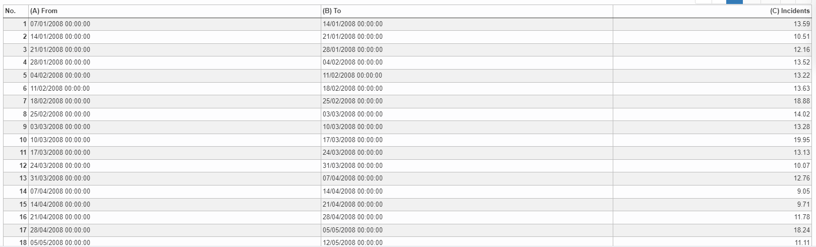
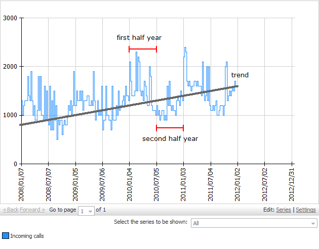
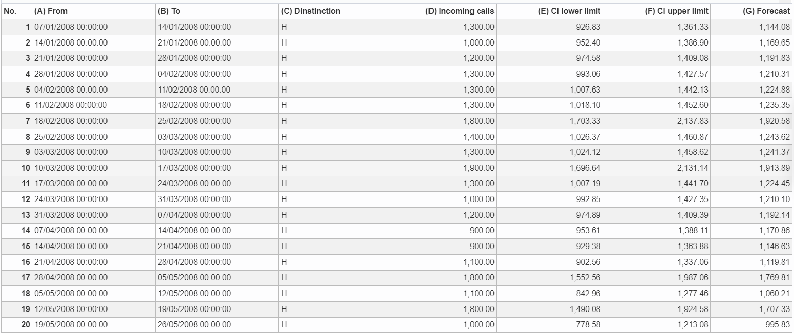
We consider the number of incoming phone calls at a call center over a time period. We are given the number of incoming calls for each week during the last four years.
|
|---|---|
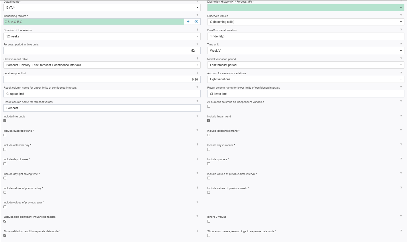
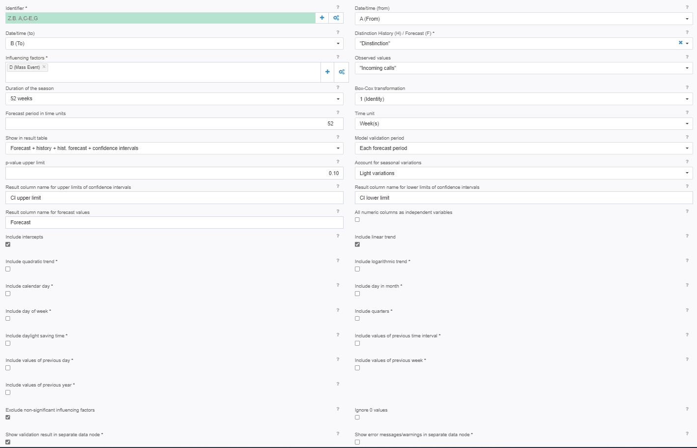
Settings |
|
Result |
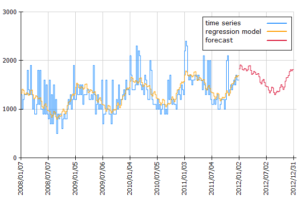
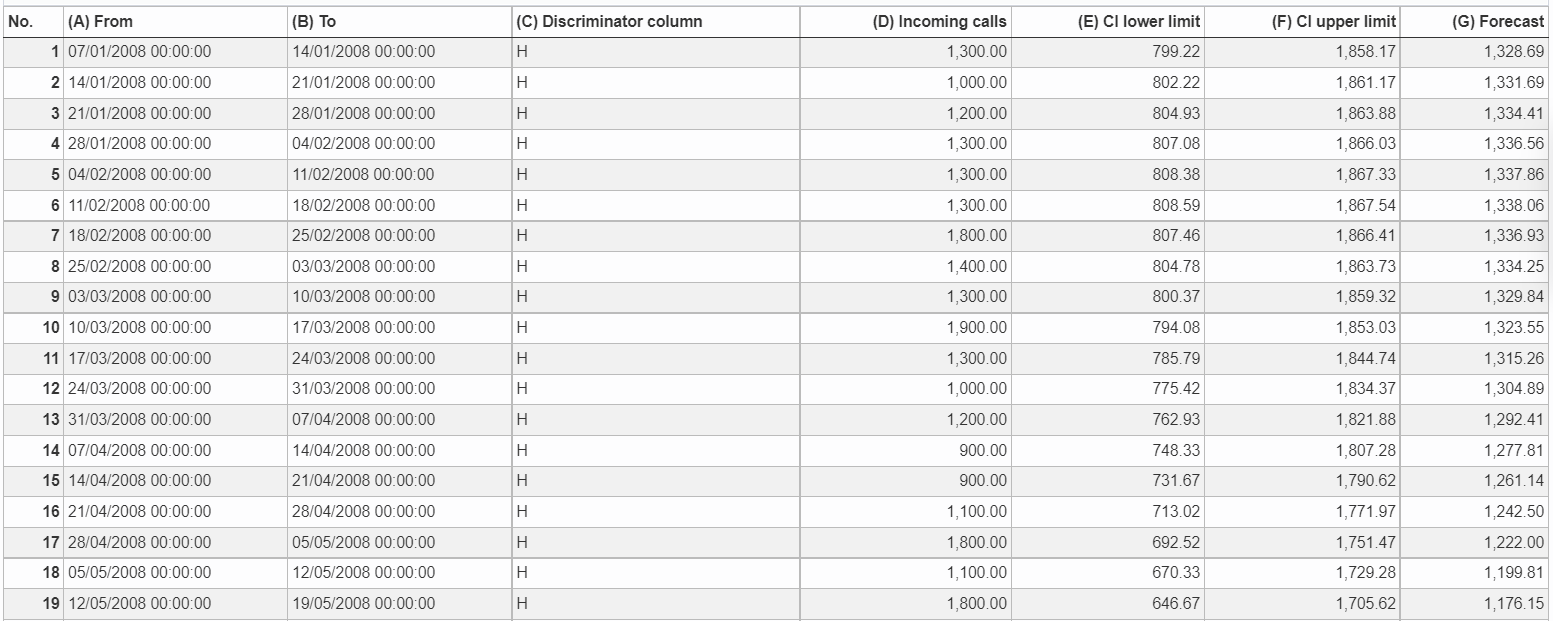
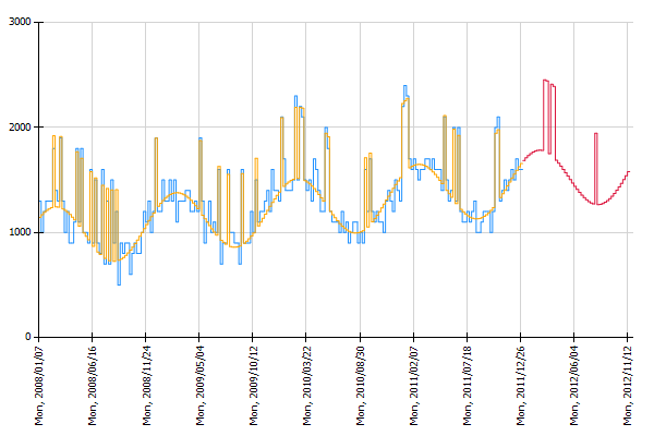
The result table shows the forecast (G), and the lower and upper limits of the confidence intervals (E and F).
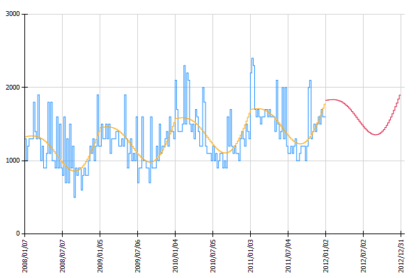
By adding a chart operation Chart: Histogram Time Pattern the visualization shows that the historical forecasts (orange line) estimated with the obtained regression model show a similar trend and seasonal behaviour as the historic observations (blue line). The red line shows the estimated number of phone calls for the next 52 weeks.
|
Project-File |
... |
Example: Regression model with trend, season and influencing factors
Situation |
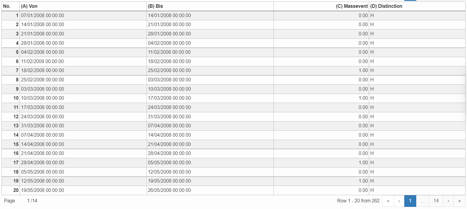
On the basis of that modified input we can now build an extended regression model. We specify advertising campaigns as an addtional influencing factor and the distinction column in the settings of the regression operation. |
|---|---|
Settings |
|
Result |
The resulting data node shows the forecast (G), and the lower and upper CI limits (E, F).
In the histogram visualizing the results (added with the operation Chart: Histogram Time Pattern) we see that campaigns could indeed explain an increased number of incoming calls in the past (compare orange and blue line). Also the forecast for the next 52 weeks (red line) contains high values whenever an advertising campaign will be run.
|
Troubleshooting
Problem |
Frequent Cause |
Solutions |
|---|---|---|
Error message: "Object reference not set to an instance of an object." |
in TIS 5.8.2, this error message occurs when the box "Output the validation result in data nodes" is checked. This is a bug, see ticket |
... |
Forecast for excluded days, e.g., holiday. |
The operator does not consider if a day in the future period is a day to be excluded or not. In our TIS Forecast solution not additional influcencing factors for days to be exlcuded are provided. If a regression model is based on at least of these influencing factor, the forecasted value for that day will be null. If a regression model does not use any additional influencing factors, e.g., they are all elminated due a high p-value, then will be a forecasted value for an excluded day. |
In the TIS forecasting solution those forecasted rows representing excluded days will be eliminated after the regression forecast (merge data, rows without a common key in data node 2). |
Month October is included in quarter 3 instead of quarter 4 |
Affects results only when option "Include quarters" is checked in TIS versions up to 6.8. This bug was fixed in TIS 6.9 |
Fixed in TIS 6.9 |